


A modular guide to simplifying complex kinetics, tracking intermediates, and deriving rate laws from molecular logic
1. Why approximation is a tool, not a shortcut
In advanced kinetics, reactions often involve multiple steps, intermediates, and feedback loops. Writing exact rate laws for these systems can be mathematically overwhelming and experimentally impractical. That’s where approximations come in.
Approximations like the steady state approximation (SSA) and the pre-equilibrium assumption allow us to simplify complex mechanisms into manageable expressions. They’re not shortcuts; they’re interpretive tools grounded in physical reasoning. They help us move from molecular behaviour to predictive equations.
This lecture focuses on SSA and its role in mechanism-to-rate law derivation. It also offers a modular recipe for turning reaction steps into rate expressions, a skill essential for chemists, biochemists, and reaction engineers.
2. What is the steady state approximation?
The SSA assumes that the concentration of a reactive intermediate remains nearly constant during the reaction. That is:
d[Intermediate]/dt ≈ 0
This doesn’t mean the intermediate is absent; it means its formation and consumption rates are balanced. The intermediate is “steady,” not static.
SSA is valid when:
- The intermediate is highly reactive
- It’s consumed as fast as it’s formed
- Its concentration is low and stable
- The system is far from equilibrium
SSA is especially useful for:
- Enzyme kinetics
- Chain reactions
- Photochemical processes
- Catalytic cycles
It allows us to eliminate intermediate concentrations from the rate law, expressing everything in terms of observable species.
3. A classic example: A → B → C
Consider a two-step consecutive reaction:
A → B → C
Let k₁ be the rate constant for A → B, and k₂ for B → C. If k₂ ≫ k₁, B is consumed as soon as it forms. Its concentration remains low and nearly constant.
Reaction Scheme
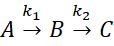
- Step 1: A → B (fast)
- Step 2: B → C (slow, rate-determining)
Steady-State Approximation for the Intermediate B
Assume that [B] quickly reaches a quasi-steady concentration, so:
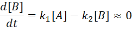
Solving for [B]:

Rate of Product Formation
The rate of formation of C depends on the slow step:

Key Point:
- The overall rate law is first-order in A,
- Governed by the slowest (rate-determining) step,
- Even though the mechanism involves two steps.
4. SSA in enzyme kinetics
In Michaelis–Menten kinetics:
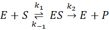
- E = free enzyme
- S = substrate
- ES = enzyme-substrate complex (intermediate)
- P = product
Step 1: Apply SSA to ES
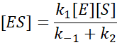
Assume the intermediate [ES] reaches steady state quickly, so:

Solve for [ES]:
Step 2: Rate of Product Formation
The rate is determined by the conversion of ES to product:

Step 3: Express [E] in Terms of Total Enzyme
Let the total enzyme be [E]₀.

Substitute [E] = [E]₀ − [ES] into the expression for v and solve for v in terms of [S]. This leads to the Michaelis–Menten equation:

Where:
- Vₘₐₓ = k₂ [E]₀
- Kₘ = (k₋₁ + k₂) / k₁
Key Insights:
- The steady-state approximation (SSA) simplifies the derivation by avoiding the need to solve coupled differential equations exactly.
- The rate law naturally shows saturation kinetics:
- At low [S]: v ∝ [S] (first-order)
- At high [S]: v → Vₘₐₓ (zero-order)
- Matches experimental behaviour of enzymes across a wide range of substrate concentrations.
This leads to the Michaelis–Menten equation after expressing [E] in terms of total enzyme concentration. SSA simplifies the derivation and reproduces the observed enzyme kinetics.
5. SSA in chain reactions
In radical chain reactions, intermediates like ·OH or ·O· are highly reactive and short-lived. Their concentrations remain low and steady, ideal for SSA.
For example, in the hydrogen–oxygen mechanism:
H· + O₂ → ·OH + ·O·
·O· + H₂ → ·OH + H·
Apply SSA to ·O·:
d[·O·]/dt = formation – consumption ≈ 0
Solve for [·O·], substitute into propagation steps, and derive the overall rate law. This helps predict explosion limits, ignition delays, and branching behaviour.
6. SSA vs. pre-equilibrium: a brief contrast
While SSA assumes intermediates are reactive and steady, pre-equilibrium assumes they’re stable and equilibrated. For example:
A + B ⇌ C → D
If k₋₁ ≫ k₂, the equilibrium between A, B, and C is fast. We assume:
[C] = K₁A][B]
Then:
v = k₂[C] = k₂K₁A][B]
Both approximations simplify the rate law, but they reflect different physical regimes. SSA is for reactive intermediates; pre-equilibrium is for stable ones.
7. Mechanism-to-rate law recipe
Here’s a modular recipe for deriving a rate law from a multi-step mechanism:
Step 1: Identify intermediates
List all species that are formed and consumed during the reaction but do not appear in the overall equation.
Step 2: Write elementary rate laws
For each step, write the rate expression using known rate constants and concentrations.
Step 3: Apply SSA to intermediates
Set d[Intermediate]/dt ≈ 0 and solve for the intermediate concentration.
Step 4: Write the overall rate
Choose a product or reactant whose rate you want to track. Express its rate in terms of intermediate concentrations.
Step 5: Substitute and simplify
Insert the SSA expressions into the overall rate. Eliminate intermediates and express the rate law in terms of observable species.
Step 6: Interpret
Determine the reaction order, rate-determining step, and limiting behaviour. Compare with experimental data.
This recipe turns molecular logic into a mathematical prediction, bridging mechanism and measurement.
8. A worked example: A + B → C via intermediate I
Mechanism:
A + B → I (k₁)
I → C (k₂)
Reaction Scheme
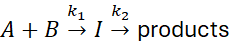
- I = reactive intermediate
- Step 1: Formation of I (fast)
- Step 2: Conversion of I to product (slow)
Step 1: Apply SSA to the intermediate I
Assume [I] reaches steady state quickly, so:
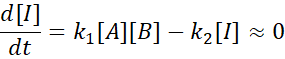
Solve for the intermediate concentration:
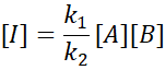
Step 2: Overall Rate of Product Formation
The rate is determined by the decay of the intermediate:

Key Insights
- The overall rate law depends only on the slowest step or effective rate constant, even though the mechanism involves an intermediate.
- The observed rate is second-order, proportional to [A] [B], despite the multi-step mechanism.
- This approach justifies using SSA to simplify complex kinetic schemes and derive experimentally observed rate laws.
So, the rate law is second-order even though the second step is unimolecular. The slow formation of I controls the rate.
9. When SSA fails
SSA is powerful, but not universal. It fails when:
- The intermediate accumulates significantly
- The system is near equilibrium
- The intermediate is long-lived or stable
- The reaction is autocatalytic or oscillatory
In such cases, full kinetic modelling is required using differential equations, numerical integration, or computational simulation.
SSA is a tool, not a law. It must be justified by physical reasoning and validated by data.
10. Summary and what’s next
The steady state approximation is a cornerstone of advanced kinetics. It simplifies complex mechanisms, clarifies intermediate behaviour, and enables mechanism-to-rate law derivation. It’s used in enzyme kinetics, chain reactions, catalysis, and beyond.
Understanding SSA means understanding how reactions unfold, not just how they’re measured. It’s a bridge between molecular choreography and mathematical expression.
In Lecture 8, we’ll explore Domino Reactions and Tandem Organic Synthesis, including how cascade mechanisms produce complexity from simplicity, and how stereochemistry and reactivity are choreographed in single-step sequences.
Support the Archive
This archive is freely shared as a communal act of care.
If you’d like to support its continuation, consider purchasing a companion PDF set for £1 per lecture via Payhip, with the final price depending on the number of lectures in the set, available only once the full series is complete.