A modular guide to overlapping pathways, intermediate behaviour, and how complex mechanisms shape rate laws

1. Why mechanism matters more than maths

In advanced kinetics, the goal isn’t just to solve equations; it’s to understand how molecules behave. Mechanisms tell us which steps occur, in what order, and how intermediates influence the overall rate. They help us interpret experimental data, predict outcomes, and design better systems.

This lecture explores three key types of complex mechanisms:

• Competitive (parallel)
• Consecutive (chain)
• Pre-equilibrium (reversible initiation)

Each produces distinctive rate laws and concentration profiles. Each also invites us to think mechanistically, not just mathematically.

2. Competitive (parallel) reactions

In a competitive mechanism, a single reactant A can follow two or more pathways simultaneously:

A → B
A → C

Each pathway has its own rate constant (k₁ and k₂), and the products B and C compete for formation. At any moment, the rate of disappearance of A is the sum of both pathways:

–d[A]/dt = k₁[A] + k₂[A]

This simplifies to:

[A] = [A]₀ · exp(–(k₁ + k₂)t)

The concentrations of B and C depend on their respective rate constants:

where:

• [A]₀ = initial concentration of A
• k₁, k₂ = first-order rate constants for the two pathways
• t = time

This shows that the ratio of B to C is constant over time, determined by the relative rates, not the absolute time or concentration.

3. Interpreting competitive behaviour

Competitive reactions are common in:

• Organic synthesis: regioselectivity and stereoselectivity
• Enzyme kinetics: multiple substrates or inhibitors
• Atmospheric chemistry: pollutant degradation
• Industrial processes: side-product formation

They help explain:

• Yield distribution
• Selectivity control
• Reaction optimisation

By adjusting conditions (e.g., temperature, solvent, catalyst), chemists can favour one pathway over another, steering the reaction toward desired products.

4. Consecutive (chain) reactions

In a consecutive mechanism, a reactant A forms an intermediate B, which then forms product C:

A → B → C

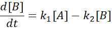
Each step has its own rate constant (k₁ and k₂), and the concentration of B builds up and decays over time. The rate equations are:

Solutions

1. For A:

2. For B:

3. For C:

Key Features

1. The sum of concentrations is conserved:

2. Behaviour at limits:

• t → 0: [A] ≈ [A]₀, [B] ≈ 0, [C] ≈ 0
• t → ∞: [A] → 0, [B] → 0, [C] → [A]₀

3. B shows a maximum at some intermediate time t₍max₎, which can be found by setting d[B]/dt = 0.

These expressions show how B peaks and then declines, while C rises steadily. The shape of the curves depends on the relative values of k₁ and k₂.

5. Case 1: k₁ ≫ k₂

If the first step is fast and the second is slow, B accumulates quickly and decays slowly. The rate-determining step is the conversion of B to C.

This is common in:

• Enzyme catalysis with slow turnover
• Gas-phase reactions with stable intermediates
• Polymerisation with slow chain termination

In this case, the overall rate is governed by k₂, the bottleneck.

6. Case 2: k₂ ≫ k₁

If the second step is fast and the first is slow, B is consumed as soon as it forms. Its concentration remains low and nearly constant, a classic steady state.

This is common in:

• Photochemical reactions
• Radical cascades
• Surface catalysis

Here, the overall rate is governed by k₁, the rate of intermediate formation.

7. Steady state approximation revisited

The steady state approximation (SSA) assumes that the concentration of a reactive intermediate remains nearly constant during the reaction. Mathematically:

d[B]/dt ≈ 0

This simplifies the rate equations and allows us to express [B] in terms of [A] and known constants. SSA is valid when:

• The intermediate is highly reactive
• It’s consumed as fast as it’s formed
• Its concentration is low and stable

SSA is used in:

• Enzyme kinetics
• Chain reactions
• Photochemistry
• Catalysis

It’s a powerful tool for simplifying complex mechanisms, but it must be applied with care.

8. Pre-equilibrium mechanisms

In a pre-equilibrium mechanism, the first step is reversible and fast, establishing an equilibrium before the second (rate-determining) step occurs:

A + B ⇌ C → D

Here, C is the intermediate, and the overall rate depends on its concentration, which is governed by the equilibrium between A and B.

Assuming k₋₁ ≫ k₂, we apply the pre-equilibrium approximation:

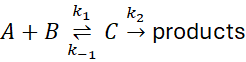
• Step 1: Formation of intermediate (fast, reversible)

• Step 2: Conversion of to product (slow, rate-determining)

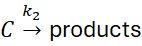
Pre-equilibrium Approximation

Assume step 1 reaches equilibrium quickly, so:

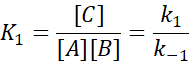
Then the concentration of the intermediate:

Overall Rate

The rate is determined by the slow step (step 2):

Key Point:

• Although the mechanism involves three steps (forward, backward, and rate-determining step), the overall rate law is second order:

• This matches experimental observations and explains why the observed kinetics do not directly show the intermediate .

Summary

Concept	Expression
Pre-equilibrium constant	K₁ = k₁ / k₋₁ = [C] / ([A][B])
Intermediate concentration	[C] = K₁ [A][B]
Overall rate	v = k₂ [C] = k₂ K₁ [A][B]
Apparent order	Second-order, even with a multi-step mechanism

9. SSA vs. pre-equilibrium: when to use which

Both SSA and pre-equilibrium simplify complex mechanisms, but they apply in different regimes.

Use SSA when:

• The intermediate is reactive
• It’s consumed rapidly
• Its concentration is low and stable

Use pre-equilibrium when:

• The first step is reversible and fast
• The intermediate is stable
• An equilibrium is established before the rate-determining step

In some cases, both approximations yield similar rate laws, but the underlying assumptions differ. Choosing the right one depends on experimental data, mechanistic insight, and kinetic behaviour.

10. Summary and what’s next

Competitive, consecutive, and pre-equilibrium mechanisms reveal the diversity of reaction pathways. They show how overlapping steps, intermediate behaviour, and kinetic assumptions shape rate laws and concentration profiles.

Understanding these mechanisms helps chemists interpret data, design experiments, and predict outcomes. It also teaches the art of simplification, reducing complexity without losing insight.

In Lecture 7, we’ll explore Steady State Approximation and Mechanism-to-Rate Law Recipes, including how to systematically derive rate laws from multi-step mechanisms using SSA and other tools.

Support the Archive

This archive is freely shared as a communal act of care.

If you’d like to support its continuation, consider purchasing a companion PDF set for £1 per lecture via Payhip, with the final price depending on the number of lectures in the set, available only once the full series is complete.